
Statistical Distribution
A statistical distribution is a mathematical description of how the values of a variable are distributed within a data set and thus represents the frequency with which each value of a variable occurs within a sample.
The most famous bell-shaped distribution is called the normal distribution, or Gauss distribution (named after German mathematician Carl Friedrich Gauss).
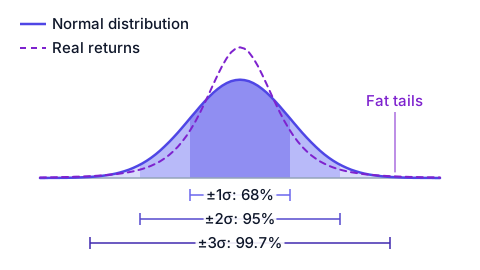
In probability theory normal distribution is a continuous probability distribution that is often used as a first approximation to describe real-valued random variables that tend to concentrate around a single mean value.
The graph of such a mathematical function is symmetric and has a bell shape, known as a "bell curve," "normal curve," or "Gaussian curve". That function is defined by the mean and standard deviation of the statistical sample analyzed. A given set of values (e.g., financial prices in a specific market) might be normal: a normality test can be used to determine this.
Standard deviation is an index of statistical variability. It is used precisely to measure how far statistical units are from the mean.
The mean, infact, unlike the standard deviation, is a positional statistical index: it is used to measure the center of gravity of the distribution but by itself is not sufficient to adequately describe the distribution of a quantitative variable. It tells you nothing, in fact, about the variability of the data. In practice, the standard deviation summarizes the deviations from the mean.
The minimum value the standard deviation can take is zero (there is no variability among the data).
When the distribution has a bell shape, the mean square deviation has a more precise interpretation (applies only to approximately symmetrical unimodal distributions, i.e. only one central peak, with a bell shape):
about 68% of observations fall within 1 standard deviation of the mean;
about 95% of observations fall within 2 standard deviation of the mean;
about 99% of observations fall within 3 standard deviation of the mean.
Those three figures belong to the normal distribution, not to markets, and the difference is not academic. Under a normal distribution a move beyond three standard deviations carries a probability of roughly 0.27 percent, which across 252 trading sessions works out to fewer than one such day per year. On real market returns those days arrive several times more often than that, and the worst single sessions in market history sit so many standard deviations away that the normal model assigns them a probability indistinguishable from zero. This is why the same quantity can be computed in two ways: against the theoretical bell curve, or against the frequencies actually observed in the data. On the same series the two answers differ, and the gap between them is precisely the risk the bell curve does not see.